What is Inference Parallelism and How it Works

In recent years, we’ve witnessed two recurring trends: the release of increasingly powerful GPUs and the introduction of Large Language Models (LLMs) with billions or trillions of parameters and expansive context windows. Many businesses are leveraging these LLMs by fine-tuning them or building out apps with domain-specific knowledge using RAG and deploying them on dedicated GPU servers. Now, when it comes to deploying these models on GPU, one thing to notice is the model size, i.e., the space required (for storing the parameters and context tokens) to load the model into the GPU memory is too high compared to the memory available on the GPU.
Model Size vs GPU Memory
There are methods to reduce model sizes by using optimization techniques like quantization, pruning, distillation & compression, etc. But if you notice in the below comparison table between the latest GPU memory and space requirement for 70B models (FP16 quantized), it’s almost impossible to handle multiple requests at a time, or in some GPUs, the model will not even fit on the memory.
| GPU | FP16 (TFLOPS) with sparsity | GPU Memory (GB) |
|---|---|---|
| B200 | 4500 | 192 |
| B100 | 3500 | 192 |
| H200 | 1979 | 141 |
| H100 | 1979 | 80 |
| L4 | 242 | 24 |
| L40S | 733 | 48 |
| L40 | 362 | 48 |
| A100 | 624 | 80 |
This is all with already applied FP16 quantization that incurs some loss of precision (which is usually acceptable in many of the generic use cases).
| Models | KV Cache in GB for Parameters (FP16) |
|---|---|
| llama3-8B | 16 |
| llama3-70B | 140 |
| llama-2-13B | 26 |
| llama2-70B | 140 |
| mistral-7B | 14 |
This brings us to the context of this blog post, i.e. how enterprises run large billion or trillion parameters LLM models on these modern datacenter GPUs. Are there any ways to split these models into smaller pieces and run only what is required at the moment, or can we distribute the parts of the model into different GPUs? I will try to answer these questions in this blog post with the current set of methods available to perform inference parallelization and also will try to highlight some of the tools/libraries that support these methods of parallelization.
Inference parallelism
Inference parallelism aims to distribute the computational workload of AI models, particularly deep learning models, across multiple processing units such as GPUs. This distribution allows for faster processing, reduced latency, and the ability to handle models that exceed the memory capacity of a single device.
Four primary methods have been developed to achieve inference parallelism, each with its strengths and applications:
- Data Parallelism
- Tensor Parallelism
- Pipeline Parallelism
- Expert Parallelism
Data parallelism
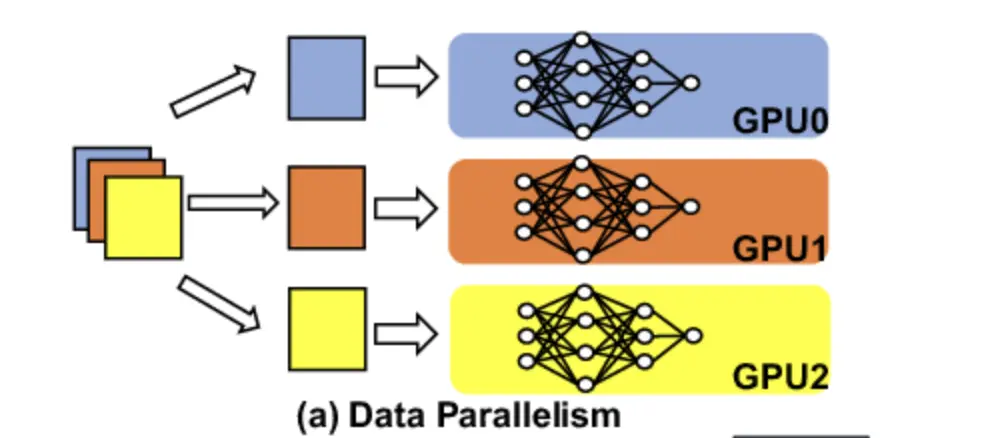
In data parallelism, we deploy multiple copies of models on different GPUs or GPU clusters. Each copy of the model independently processes the user request. In a simple analogy, this is like having multiple replicas of 1 microservice.
Now, a common question one might have is how it solves the problem of model size fitting into GPU memory, which we discussed at the start, and the short answer is that it doesn’t. This method is only recommended for smaller models that can fit into the GPU memory. In those cases, we can use multiple copies of the model deployed on different GPU instances and distribute the requests to different instances hence providing enough GPU resources for each request and also increasing the availability of the service. This will also increase the overall request throughput for the system as you have more instances to handle the traffic now.
Tensor parallelism
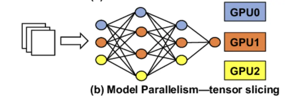
In tensor parallelism, we split each layer of the model across different GPUs. A single user request will be shared across multiple GPUs and the result of each request’s GPU computations will be recombined over a GPU-to-GPU network.
To understand it better, as the name suggests, we split the tensors into chunks along a particular dimension such that each device only holds 1/N chunk of the tensor. Computation is performed using this partial chunk to get partial output. These partial outputs are collected from all devices and then combined.
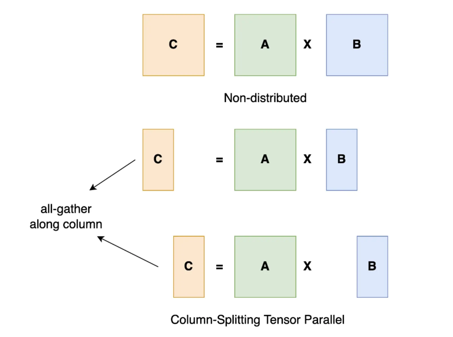
As you might have noticed already, the bottleneck to the performance of tensor parallelism is the speed of the network between GPU-to-GPU. As each request will be computed across different GPUs and then combined, we need a high-performance network to ensure low latency numbers.
Pipeline parallelism
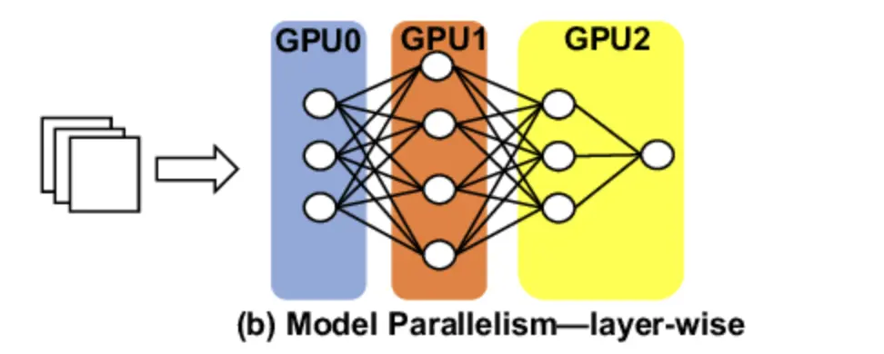
In pipeline parallelism, we distribute a group of model layers across different GPUs. Layer-based partitioning is the fundamental approach in pipeline parallelism. The model’s layers are grouped into continuous blocks, forming stages. This partitioning is typically done vertically through the network’s architecture. Computational balance is a key consideration. Ideally, each stage should have an approximately equal computational load to prevent bottlenecks. This often involves grouping layers of varying complexities to achieve balance. Memory usage optimization is another critical factor. Stages are designed to fit within the memory constraints of individual devices while maximizing utilization. Communication overhead minimization is also important. The partitioning aims to reduce the amount of data transferred between stages, as inter-device communication can be a significant performance bottleneck.
So for example, if you are deploying LLaMA3-8B model that has 32 layers on a 4 GPU instance, you can split and distribute 8 layers of model on each GPU. The processing of requests happens in a sequential manner where the computation starts at one GPU and continues to the next GPU with point-to-point communication.
Again, as multiple GPU instances are involved, the networking can become a huge bottleneck if we do not have high-speed network communication between the GPUs.This parallelism can increase the GPU throughput as every request will need fewer resources from each GPU and should be easily available, but it will end up increasing the overall latency as the request will be processed sequentially, and delay in any GPU computation or network component will cause an overall surge in latency.
Expert parallelism
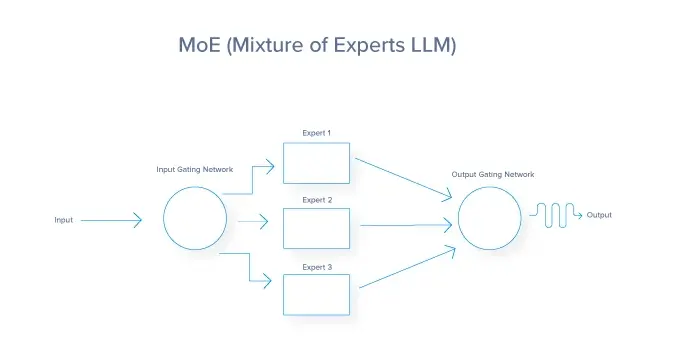
Expert parallelism, often implemented as a Mixture of Experts (MoE), is a technique that allows for the efficient use of large models during the inference process. It doesn’t solve the problem of fitting the models into the GPU memory but provides an option to have a broad capability model serving the requests based on the request context. In this technique, the model is divided into multiple expert sub-networks. Each expert is typically a neural network trained to handle specific types of inputs or subtasks within the broader problem domain. A gating network determines which expert to use for each input. Only a subset of experts is activated for any given input. Different experts can be distributed across different GPUs. Router/Gating network and active experts can operate in parallel. Inactive experts don’t consume computational resources. This greatly reduces the number of parameters that each request must interact with, as some experts are skipped. But like Tensor & Pipeline parallelism the overall request latency relies heavily on the GPU-to-GPU communication network. A request must be reconstituted back to their original GPUs after expert processing generating high networking communication over the GPU-to-GPU interconnect fabric.
This approach can lead to better utilization of hardware compared to Tensor parallelism as you don’t have to split the operations into smaller chunks.
Following is a summary and comparison of the methods we discussed. You can use it as a reference when planning to choose one for your use case.
| Aspect | Data Parallelism | Tensor Parallelism | Pipeline Parallelism | Expert Parallelism |
|---|---|---|---|---|
| Basic Concept | Splits input data across multiple devices | Splits individual tensors/layers across devices | Splits model into sequential stages across devices | Splits model into multiple expert sub-networks |
| How it Works | The same model is replicated on each device, processing different data chunks | Single layer/operation distributed across multiple devices | Different parts of the model pipeline on different devices | The router selects specific experts for each input |
| Parallelization Unit | Batch of inputs | Individual tensors/layers | Model stages | Experts (sub-networks) |
| Scalability | Scales well with batch size | Scales well for very large models | Scales well for deep models | Scales well for wide models |
| Memory Efficiency | Low (full model on each device) | High (only part of each layer on each device) | High (only part of the model on each device) | Medium to High (experts distributed across devices) |
| Communication Overhead | Low | Medium to High | Low (only between adjacent stages) | Medium (router communication and expert selection) |
| Load Balancing | Generally balanced if data is evenly distributed | Balanced within operations | Can be challenging, and requires careful stage design | Can be challenging, and requires effective routing |
| Latency | Low for large batches | Can increase for small batches | Higher due to pipeline depth | Can be low if routing is efficient |
| Throughput | High for large batches | Can be high for large models | High, especially for deep models | Can be very high for diverse inputs |
| Typical Use Cases | Large batch inference, embarrassingly parallel tasks | Very large models that don’t fit on a single device | Deep models with sequential dependencies | Models with diverse sub-tasks or specializations |
| Challenges | Limited by batch size, high memory usage | Complex implementation, potential communication bottlenecks | Pipeline bubble, difficulty in optimal stage partitioning | Load balancing, routing overhead, training instability |
| Adaptability to Input Size | Highly adaptable | Less adaptable, fixed tensor partitioning | Less adaptable, fixed pipeline | Highly adaptable, different experts for different inputs |
| Suitable Model Types | Most model types | Transformer-based models, very large neural networks | Deep sequential models | Multi-task models, language models with diverse knowledge |
| Supported Inference Backends | TensonRT-LLM, vLLM, TGI | TensonRT-LLM, vLLM, TGI | TensonRT-LLM, vLLM, TGI | TensonRT-LLM, vLLM, TGI |
Parallelism techniques combined
By now, you might already be thinking that if using the above parallelism methods means we are reducing the overall consumption or utilization of GPU, then can we not combine or replicate these to increase the overall GPU throughput? Combining Inference parallelism methods can lead to more efficient and scalable systems, especially for large and complex models.
In the table below, you can see 4 possible options but in actual scenarios based on the number of GPUs you have, this combination can grow to a very large number.
| Data Parallelism (DP) + Pipeline Parallelism (PP) | Tensor Parallelism (TP) + Pipeline Parallelism (PP) | Expert Parallelism (EP) + Data Parallelism (DP) | Tensor Parallelism (TP) + Expert Parallelism (EP) |
|---|---|---|---|
| Split the model into stages (pipeline parallelism) | Divide the model into stages (pipeline parallelism) | Distribute experts across devices (expert parallelism) | Split large expert models across devices (tensor parallelism) |
| Replicate each stage across multiple devices (data parallelism) | Split large tensors within each stage across devices (tensor parallelism) | Process multiple inputs in parallel (data parallelism) | Split large expert models across devices (tensor parallelism) |
So for example let’s say you have 64 GPU available and you are planning to deploy llama3-8b or Mistral 8*7B model on them. The following are some of the possible combinations of the parallelism methods. These are just examples to understand the parallelism combination strategies, for the actual use case you need to consider and benchmark other options as well.
LLaMA 3-8B (64 GPUs)
| Strategy | GPU Allocation | Pros | Cons |
|---|---|---|---|
| PP8TP8 | 64 = 8 (pipeline) × 8 (tensor) | - Balanced distribution - Reduced Communication | - Pipeline bubbles - Increased latency |
| PP4TP4DP4 | 64 = 4 (pipeline) × 4 (tensor) × 4 (data) | - Higher throughput - Flexible for batch sizes | - Complex integration - Requires large batches |
| DP8TP8 | 64 = 8 (data) × 8 (tensor) | - Higher throughput - No pipeline bubbles | - Large batch size needed - High memory per GPU |
Mistral 8*7B (64 GPUs)
| Strategy | GPU Allocation | Pros | Cons |
|---|---|---|---|
| EP8TP8 | 64 = 8 (experts) × 8 (tensor per expert) | - Balanced memory distribution - Efficient memory use | - Complex load balancing - Potential compute underutilization |
| EP8TP4DP2 | 64 = 8 (experts) × 4 (tensor) × 2 (data) | - Higher throughput - Balanced utilization | - Needs careful load balancing - Large batch sizes required |
| EP8PP2TP4 | 64 = 8 (experts) × 2 (pipeline) × 4 (tensor) | - Supports deeper experts - Flexible scaling | - Increased latency - Complex synchronization |
How to choose one?
Now we have covered 4 methods of Inference parallelism, and then we have multiple combinations of these methods, so a common question you might be having is how do you choose or identify which method to use. So, the choice of inference parallelism methods broadly depends on the following factors:
- Model architecture
- Use case requirements (Latency vs Throughput)
- Hardware configuration
Model architecture
Model architecture plays a crucial role in determining the most effective inference parallelism strategy. You need to identify your model architecture and then choose the parallelism method or combination of them that fits well. Different model structures fit to different parallelization techniques:
- Large, deep models (e.g., GPT-4, PaLM 2):
- Benefit from pipeline parallelism
- Can be split into stages across multiple GPUs
- Good for models with many sequential layers
- Wide models with large layer sizes (LLaMA 2, BLOOM):
- Ideal for tensor parallelism
- Allow splitting individual layers across GPUs
- Effective for models with very large matrix operations
- Ensemble models or Mixture of Experts (Mixtral 8x7B, Switch Transformers):
- Well-suited for expert parallelism
- Different experts can be distributed across GPUs
- Useful for models that use different sub-networks for various tasks
- Models with small computational graphs (GPT-3.5-turbo, Falcon-7B):
- Often works well with simple data parallelism
- Can replicate the entire model across GPUs
- Effective when the model fits entirely in GPU memory
- Attention-based models (e.g., Transformers):
- Can benefit from attention slicing or multi-head parallelism
- Allow distributing attention computations across GPUs
Use case requirements (Latency vs Throughput tradeoff)
You need to be familiar with your business requirements or use case, i.e., what matters to business more, the latency of the user requests, or utilization of the GPU. Or can you identify the mode of your application i.e., is it a real-time application where response time to the user request is the main driver for the user experience, or is it an offline system where response time to the user request is not the primary concern
The reason we need to be aware of this is the tradeoff between latency and GPU throughput. If you want to reduce the latency to the user request you need to allocate more GPU resources to each request and your choice of parallelism method will rely on that. You can do optimal batching so that requests are not struggling to acquire the GPU resource which increases the overall latency.
However, if latency is not the consideration, then your goal should be to achieve maximum throughput on the GPU by choosing the right parallelism method and appropriate batch sizes that utilize GPU resources to its maximum throughput.
| Use Case | Preferred Parallelism | Latency vs Throughput Consideration |
|---|---|---|
| Real-time chatbots | Data parallelism or Tensor parallelism | Low latency priority; moderate throughput |
| Batch text processing | Pipeline parallelism | High throughput priority; latency less critical |
| Content recommendation | Expert parallelism | High throughput for diverse inputs; moderate latency |
| Sentiment analysis | Data parallelism | High throughput; latency less critical for bulk processing |
| Voice assistants | Tensor parallelism or Pipeline parallelism | Very low latency priority; moderate throughput |
Hardware configuration
Hardware configuration often dictates the feasible parallelism strategies, and the choice should be optimized for the specific inference workload and model architecture. Following are some hardware component choices that impact the overall parallelism choices.
| Hardware Component | Impact on Parallelism Choice | Examples |
|---|---|---|
| GPU Memory Capacity | Determines feasibility of data parallelism and influences the degree of model sharding | NVIDIA A100 (80GB) allows larger model chunks than A100 (40GB) |
| Number of GPUs | Affects the degree of parallelism possible across all strategies | 8 GPUs enable more parallelism than 4 GPUs |
| GPU Interconnect Bandwidth | Influences efficiency of tensor and pipeline parallelism | NVLink offers higher bandwidth than PCIe, benefiting tensor parallelism |
| CPU Capabilities | Impacts data preprocessing and postprocessing in parallelism strategies | High-core count CPUs can better handle data parallelism overhead |
| System Memory | Affects the ability to hold large datasets for data parallelism | 1TB system RAM allows larger batch sizes than 256GB |
| Storage Speed | Influences data loading speeds in data parallelism | NVMe SSDs provide faster data loading than SATA SSDs |
| Network Bandwidth | Critical for distributed inference across multiple nodes | Networks based on Infiniband, RoCE are faster than conventional networks for GPU fabrics |
| Specialized Hardware | Enables specific optimizations | Google TPUs are optimized for tensor operations |
Conclusion
AI inference parallelism is a game-changer for running big AI models efficiently. We’ve looked at different ways to split up the work, like data parallelism, tensor parallelism, pipeline parallelism, and expert parallelism. Each method has its own pros and cons, and choosing the right one depends on your specific needs and setup. It’s exciting to see tools like TensorRT-LLM, vLLM, and Hugging Face’s Text Generation Inference making these advanced techniques easier for more people to use. As AI models keep getting bigger and more complex, knowing how to use these parallelism techniques will be super important. They’re not just about handling bigger models – they’re about running AI smarter and more efficiently. By using these methods well, we can do amazing things with AI, making it faster, cheaper, and more powerful for all kinds of uses.
The future of AI isn’t just about bigger models; it’s about finding clever ways to use them in the real world. With these parallelism techniques, we’re opening doors to AI applications that were once thought impossible. If you’re looking for experts who can help you scale or build your AI infrastructure, reach out to our AI & GPU Cloud experts.
If you found this post valuable and informative, subscribe to our weekly newsletter for more posts like this. I’d love to hear your thoughts on this post, so do start a conversation on LinkedIn.
References
Stay updated with latest in AI and Cloud Native tech
We hate 😖 spam as much as you do! You're in a safe company.
Only delivering solid AI & cloud native content.

